SIIM-ACR Pneumothorax Segmentation
Identify Pneumothorax disease in chest x-rays

Table of Contents
- Introduction
- Business Problem
- Business objectives and constraints
- Data overview and Data set column analysis
- Mapping the real world problem to a Machine Learning Problem
- Performance metric
- Exploratory Data Analysis
- Existing Solutions/Approaches
- First cut approach
- Preprocessing
- Model building
- Inference Pipeline
- Deployment
- Summary
- Future Work
- Profile
- References
1. Introduction
What Is a Collapsed Lung (Pneumothorax)?
A collapsed lung or Pneumothorax refers to a condition in which the space between the wall of the chest cavity and the lung itself fills with air, causing all or a portion of the lung to collapse. Air usually enters this space, called the pleural space, through an injury to the chest wall or a hole in the lung. This result is called a Pneumothorax, which is the medical term for a collapsed lung.
What Causes a Collapsed Lung?
Causes of collapsed lung include trauma to the chest cavity (fractured rib, penetrating trauma from a bullet, knife, or other sharp object), cigarette smoking, drug abuse, and certain lung diseases. Sometimes, the lung may collapse without an apparent injury, called spontaneous Pneumothorax.
What Are the Signs and Symptoms of a Collapsed Lung?
Symptoms of collapsed lung include sharp, stabbing chest pain that worsens on breathing or with deep inhalation that often radiates to the shoulder and or back; and a dry, hacking cough. In severe cases a person may go into shock, which is a life-threatening condition that requires immediate medical treatment. See a doctor for any type of chest pain or suspected Pneumothorax.
How Is a Collapsed Lung Treated?
A small Pneumothorax without underlying lung disease may resolve on its own in one to two weeks.however a large Pneumothorax is usually treated with removal of air under pressure, by inserting a needle attached to a syringe into the chest cavity. A chest tube may be used and left in place for several days. In some cases, surgery may be needed.
Who is at risk for Pneumothorax?
- Sometimes, very tall, thin people are prone to a spontaneous Pneumothorax. In this condition, the lung collapses after minimal or no trauma.
- Spontaneous Pneumothorax is more common in smokers and in men between the ages of 20 and 40. Smoking has been shown to increase the risk for spontaneous Pneumothorax.
For more information and clear understanding you can refer to this video
2. Business/Real-world Problem

Imagine suddenly gasping for air, helplessly breathless for no apparent reason. Could it be a collapsed lung?
Pneumothorax can be caused by a blunt chest injury, damage from underlying lung disease, or most horrifying — it may occur for no obvious reason at all. On some occasions, a collapsed lung can be a life-threatening event.
Pneumothorax is usually diagnosed by a radiologist on a chest x-ray, and can sometimes be very difficult to confirm. An accurate AI algorithm to detect Pneumothorax would be useful in a lot of clinical scenarios. AI could be used to triage chest radio graphs for priority interpretation, or to provide a more confident diagnosis for non-radiologists.
The Society for Imaging Informatics in Medicine (SIIM) is the leading healthcare organization for those interested in the current and future use of informatics in medical imaging. Their mission is to advance medical imaging informatics across the enterprise through education, research, and innovation in a multi-disciplinary community.
In this competition, we’ll develop a model to classify (and if present, segment) Pneumothorax from a set of chest radio graphic images. If successful, we could aid in the early recognition of Pneumothoraces and save lives.

It requires a lot of effort to determine certain cases of Pneumothorax where the affected area is minimal and it also requires good domain experts. So having an AI enabled system will help radiologists by reducing the time required to run diagnostic tests and also reduce the chances of errors. The algorithm had to be extremely accurate because lives of people is at stake.
3. Business objectives and constraints
Objectives:
- We need to predict Pneumothorax from a set of chest radio graphic images and if it is present we need to segment that also
- Minimize Dice coefficient.
Constraints:
1. Since it's a medical domain problem so predicting False Negatives          is a big issue.
2. No strict latency constraints.
3. Data overview and Data set column analysis
Data Source:
Originally the data set was available to download using Google Cloud Healthcare AP. The API is not currently functional since most people have already shared it.Thanks to See — for making the data easily accessible. I have used Kaggle API to download the data to my Google Drive.
After we download the dateset, it is important to understand the hierarchy or folder structure of the images.

We have images separated in a test and train folder, train-rle.csv is the class label file.

The format of images is .dcm format. We need to understand the terminology below to solve the problem.
What is the DICOM format?
DICOM is an abbreviation for Digital Imaging and Communications in Medicine. It is a standard format for storing, printing and transmitting information in medical imaging. This format is used worldwide. DICOM format is represented as “.dcm”.
What does DICOM format contain?
DICOM contains image data along with other important information about the patent demographics, and study parameters such as patient name, patient id, patient age and patient weight. For confidentiality purposes, all information that identifies the patient is removed before transmitting it for educational or research purposes.
How to read and extract data from DICOM format in python?
You can read DICOM files in python using pydicom library. You can refer to the official Github page for more information about extracting data from DICOM files. Here is link
What Is Run-length encoding (RLE) ?
Run-length encoding (RLE) is a very simple form of lossless data compression.
This video on YouTube explains how it works. This competition provides a separate CSV file with encodings for each image, which annotates or labels the segment of the image consisting Pneumothorax. However, images without Pneumothorax have a mask value of -1.
What is PA and AP View Position?
A PA chest radio graph is taken with the x-ray tube behind the patient such that the x-rays enter from the posterior (P) of the patient and exit from the anterior (A) of the patient. The detector is anterior to the patient. AP radio graphs are taken with the tube in front of the patient with the detector behind the patient. These are usually done with portable equipment and the patient is typically in bed.
What is modality
Modality is the term used in radiology to refer to one form of imaging e.g. CT scanning
4. Mapping the real world problem to a Machine Learning Problem
Type of Machine Learning Problem:
We are attempting to predict the existence of pneumothorax in our test images and
indicate the location and extent of the condition using masks.
So this is a classification and image segmentation problem. In the Classification phase we will classify if the image has Pneumothorax
or not and in segmentation phase we will locate the affected area using Semantic Segmentation.
Our model should create binary masks and encode them using RLE.
Let us have an overview of Image Segmentation
What is Image Segmentation?
In digital image processing and computer vision, image segmentation is the process of partitioning a digital image into multiple segments (sets of pixels, also known as image objects). More precisely, image segmentation is the process of assigning a label to every pixel in an image such that pixels with the same label share certain characteristics.
Object detection vs Image Segmentation
Object detection builds a bounding box corresponding to each class in the image. But it tells us nothing about the shape of the object. We only get the set of bounding box coordinates. Image segmentation creates a pixel-wise mask for each object in the image. This technique gives us a far more granular understanding of the object(s) in the image.
Why do we need Image Segmentation?
The shape of the cancerous cells plays a vital role in determining the severity of the cancer. You might have put the pieces together — object detection will not be very useful here. We will only generate bounding boxes which will not help us in identifying the shape of the cells.

Image Segmentation techniques make a MASSIVE impact here. it helps us approach this problem in a more granular manner and get more meaningful results. A win-win for everyone in the healthcare industry.Here, we can clearly see the shapes of all the cancerous cells.
There are many other applications where Image segmentation is transforming industries:
- Traffic Control Systems
- Self Driving Cars
- Locating objects in satellite image and many more
The Different Types of Image Segmentation
- Semantic Segmentation: The goal of semantic image segmentation is to label each pixel of an image with a corresponding class of what is being represented.it is kind of a pixel level image classification.
- Instance segmentation: Instance segmentation is one step ahead of semantic segmentation wherein along with pixel level classification, we expect the computer to classify each instance of a class separately.
If you are still confused between the differences of object detection, semantic segmentation and instance segmentation, below image will help to clarify the point:

6. Performance metric:
- Dice coefficient
The Dice coefficient can be used to compare the pixel-wise agreement between a predicted segmentation and its corresponding ground truth. The formula is given by:

2. Recall :
Recall calculates the percentage of actual positives a model correctly identified (True Positive). When the cost of a false negative is high, we should use recall.

Loss Used : We are using a combined loss as described below
combined_loss = Dice Loss + BCE
BCE is binary cross entropy and Dice Loss is (1- Dice coefficient)
7. Exploratory Data Analysis:
Sample Image from data set

In the left image the portion with disease is highlighted with red mask and one bounding box . The right image is without mask but with bounding box. It is really hard to identify the disease with open eyes for common people.
There are lot of meta data associated with the .DICOM files. But for analysis we are extracting some of the important info from the files.
Number of images in train vs test data

Observation : There are 12089 files in train data and 3205 files in test data
Class distribution in train data

Observation : The data is imbalanced and there are only 27.6% of positive cases.
Gender wise data distribution

Observation There are more male person data than female person
Disease distribution across Gender

Observation Men and women are equally likely to be affected by Pneumothorax.
Age wise Pneumothorax distribution

Observation The above diagram clearly shows people from different ages can be affected by Pneumothorax. However as per data set people of age 51 is highly affected by the the disease than others.
Box plot of Age vs Class

Observation Similar conclusions as above can be drawn here.People of all ages can be affected by the disease. We can clearly see 2 outliers in the age 148 and 413.
The presence of Pneumothorax at particular ages and genders

Observation The healthy people distribution is very similar to Gaussian distribution but not exactly same. Men of age 15 are affected as men of age 65.
View_position wise data distribution

Observation There are more X-ray images done in PA position than AP which is quite natural as if PA is not possible for a patient due some reason then doctors prefer to do AP.
Analyzing The Affected Area
In the metadata of images we don’t have the area affected by Pneumothorax. However from the masking information we can approximate the area. We convert RLE encoded masks to image form.Then we will count the non zero elements in this array to count the number of pixels we have. Pixel spacing gives us the length and width of patient’s chest per pixel. We will multiply the area per pixel driven of pixel spacing by total number of pixels to get an estimation of the affected area in sq mm.
Box plot of Affected area vs Sex

Observation It is clear that the affected area for Men is more than Females as median, Q3, IQR, end whisker are larger for men than females. There are lot of outliers also for both cases.
Let us divide the people in different age categories and see how the disease affects different age groups
Box plot of Affected area vs Age Category

Observation For youth the affected area is higher as median is higher. For children the affected area is smaller than others. Except seniors the IQR for male is higher than females.
8. Existing Solutions/Approaches
- Model: UNet.
- Backbone: ResNet34 backbone with frozen batch-normalization.
- Preprocessing: training on random crops with (512, 512) size, inference on (768, 768) size.
- Augmentations: ShiftScaleRotate, RandomBrightnessContrast, ElasticTransform, HorizontalFlip from albumentations.
- Optimizer: Adam, batch_size=8
- Scheduler: CosineAnnealingLR
- Additional feature: the proportion of non-empty samples linearly decreased from 0.8 to 0.22 (as in train dataset) depending on the epoch. It helped to converge faster.
- Loss: 2.7 * BCE(pred_mask, gt_mask) + 0.9 * DICE(pred_mask, gt_mask) + 0.1 * BCE(pred_empty, gt_empty).
- Here pred_mask is the prediction of the UNet, pred_empty is the prediction of the branch for empty mask classification.
Approach2: Nested Unet With EfficientNet encoder

Unet plus plus introduces intermediate layers to skip connections of U-Net, which naturally form multiple new up-sampling paths from different depths, ensembling U-Nets of various receptive fields. This results in far better performance than traditional Unet.
- Model : Unet
- Backbone : EfficientNet B4 Encoder initialized with ‘Imagenet’ weights
- Augmentations : HorizontalFlip , RandomContrast, RandomGamma, RandomBrightness, ElasticTransform, GridDistortion, OpticalDistortion, RandomSizedCrop from albumentations.
- Loss : Dice loss + BCE loss
- Metrics : IOU( intersection over union)
- Optimizer: Adam, batch_size=16
- Dropout rate : 0.5
- Learning rate Scheduler: CosineAnnealingLR
- Image_size = 256,256,16
9. First cut approach:

We are going to apply Convolutional neural network based deep neural networks to analyze the image data. Convolutional networks were inspired by biological processes in that the connectivity pattern between neurons resembles the organization of the animal visual cortex.
We will solve the problem in two parts. First we will build a classification model that will classify if the image has Pneumothorax or not. If present we will use a second model to segment the affected area. Here is the process flow.

To build the classification model we will apply Transfer Learning method where we use ChexNet model as a feature extractor . ChexNet is a deep learning algorithm that can detect and localize 14 kinds of diseases from chest X-ray images. As described in the paper, a 121-layer densely connected convolutional neural network is trained on ChestX-ray14 data set, which contains 112,120 frontal view X-ray images from 30,805 unique patients. The result is so good that it surpasses the performance of practicing radiologists.
We will remove the the last dense layer from ChexNet model and we will attach custom dense layers at the end and train the network.
Loss: ‘categorical_crossentropy’ since labels are one hot encoded with output labels [1 0] means Pneumothorax negative and [0 1] means vice versa.
Metric : ‘Recall’ since cost of false negative is high.
Results : The loss best loss achieved is 0.3 and recall is 0.87.

For Biomedical Image Segmentation the most popular architecture that comes in mind is UNET. In the original paper, the UNET is described as follows:

The architecture contains two paths. First path is the contraction path (also called as the encoder) which is used to capture the context in the image. The encoder is just a traditional stack of convolutional and max pooling layers. The second path is the symmetric expanding path (also called as the decoder) which is used to enable precise localization using transposed convolutions. Thus it is an end-to-end fully convolutional network (FCN). Here is the code.
Results: Best validation loss achieved is 0.93 and Dice coefficient is 0.09.

Prediction Results:

Observation: Though the model is learning but we need to do more better in terms of segmentation task. We will apply more complex models to get better performance.
10. Preprocessing
We are going extract the pixel array from DICOM files to generate the .png file corresponding to each DICOM file. We are also going to convert the RLE encode masks to .png image. While model training we will use this image files.
11. Model building:
To built models we are going to extensively use Transfer Learning. Andrew Ng, renowned professor and data scientist, who has been associated with Google Brain, Baidu, Stanford and Coursera, in one of his tutorial ‘Nuts and bolts of building AI applications using Deep Learning’ mentioned,
After supervised learning — Transfer Learning will be the next driver of ML commercial success
If are more interested you can refer this video
Framework and environment Used:
We are going to use TensorFlow 2.0 to prepare the data pipeline. To know more you can refer the tutorials page of TensorFlow.
We have used Google Colab backed with 25 GB RAM and 16 GB NVIDIA TESLA K80 GPU as our environment.
Prepare data pipeline:
We will use tf.data API of TensorFlow which uses the Extract Transform Load (ETL) format to propagate data from its source all the way into your model.
Extract: In extract phase we are going to built a mini pipeline of instructions to set Google Drive paths from where we need to read the stored image data into RAM.
Transform: In Transom stage we are going resize the image since the input image is 1024 x 1024 and we will resize it to 256 x 256 so that the data can easily fit into memory.We will read raw images as 3 Channel image and masks as 1 channel image. Here we will apply image augmentation techniques so that the model generalization ability increases on the test data.
Load: Finally We are going to load the data in batches of Size 16 and train our model since loading the entire data at once can explode our RAM. The most important feature of tf.Data API that fascinates me is prefetch functionality. What it does is, during model execution (forward and back propagation), it drives the CPU to prepare the next batch of our data set to be fed into our model immediately after training on the previous batch. This is really exciting, since it allows us to fully utilize our hardware resources and rescue our GPU from data starvation.


The Model.fit() method is going to load the data into RAM and feed it to model for training. Here is the complete pipeline code
Sample images from a single batch:
As a sanity check whether our data pipeline is working properly or not I have plotted the data from a single batch.

Different Models:
UNET with VGG 16 as backbone:
VGG16 is a convolutional neural network model proposed by K. Simonyan and A. Zisserman from the University of Oxford in the paper “Very Deep Convolutional Networks for Large-Scale Image Recognition”. The model achieves 92.7% test accuracy in ImageNet, which is a dataset of over 14 million images belonging to 1000 classes. It was one of the famous model submitted to ILSVRC-2014. It makes the improvement over AlexNet by replacing large kernel-sized filters (11 and 5 in the first and second convolutional layer, respectively) with multiple 3×3 kernel-sized filters one after another.
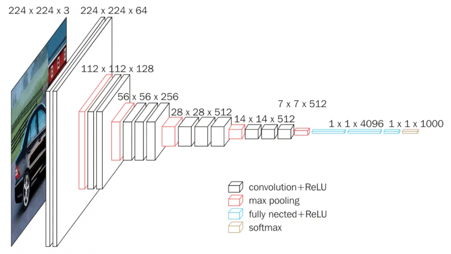
We have used VGG 16 with ‘imagenet’ weights as a encoder part and UNET’s decoder part to upsample the image to original size.
We don’t need to implement everything from scratch as we have a nice library segmentation_models to do all this tasks. All we need to do is to pass right set of arguments. Here is the code.
Results : Best validation loss is 0.87 and Dice Coefficient is 0.15

UNET with DenseNet as backbone:

DenseNet (Dense Convolutional Network) is an architecture that focuses on making the deep learning networks go even deeper, but at the same time making them more efficient to train, by using shorter connections between the layers. DenseNet is a convolutional neural network where each layer is connected to all other layers that are deeper in the network, that is, the first layer is connected to the 2nd, 3rd, 4th and so on, the second layer is connected to the 3rd, 4th, 5th and so on. This is done to enable maximum information flow between the layers of the network. To preserve the feed-forward nature, each layer obtains inputs from all the previous layers and passes on its own feature maps to all the layers which will come after it. Unlike Resnets it does not combine features through summation but combines the features by concatenating them. So the ‘ith’ layer has ‘i’ inputs and consists of feature maps of all its preceding convolutional blocks. Its own feature maps are passed on to all the next ‘I-i’ layers. This introduces ‘(I(I+1))/2’ connections in the network, rather than just ‘I’ connections as in traditional deep learning architectures. It hence requires fewer parameters than traditional convolutional neural networks, as there is no need to learn unimportant feature maps.
Results : Best validation loss is 0.85 and Dice Coefficient is 0.17

UNET with EfficientNet as backbone:
The authors proposed a simple yet very effective scaling technique which uses a compound coefficient ɸ to uniformly scale network width, depth, and resolution in a principled way:

ɸ is a user-specified coefficient that controls how many resources are available whereas α, β, and γ specify how to assign these resources to network depth, width, and resolution respectively.
In a CNN, Conv layers are the most compute expensive part of the network. Also, FLOPS of a regular convolution op is almost proportional to d, w², r², i.e. doubling the depth will double the FLOPS while doubling width or resolution increases FLOPS almost by four times. Hence, in order to make sure that the total FLOPS don’t exceed 2^ϕ, the constraint applied is that (α * β² * γ²) ≈ 2
EfficientNet-B0 : The authors used Neural Architecture Search approach similar to MNasNet research paper. This is a reinforcement learning based approach where the authors developed a baseline neural architecture Efficient-B0 by leveraging a multi-objective search that optimizes for both Accuracy and FLOPS.
The MBConv layer above is nothing but an inverted bottleneck block with squeeze and excitation connection added to it. Starting from this baseline architecture, the authors scaled the EfficientNet-B0 using Compound Scaling to obtain EfficientNet B1-B7.

Results with EfficientNet B4: Best validation loss is 0.65 and Dice Coefficient is 0.36

Results with EfficientNet B7: Best validation loss is 0.72 and Dice Coefficient is 0.29`

Final Results:
Below are the results obtained from our best model UNet with EfficientNet B4 as backbone.

12. Inference Pipeline
13. Deployment:
To deploy our model we are going to use Streamlit. Streamlit is an awesome new tool that allows engineers to quickly build highly interactive web applications around their data, machine learning models, and pretty much anything.
The best thing about Streamlit is it doesn’t require any knowledge of web development. If you know Python, you’re good to go! You can refer to their tutorials page for further knowledge.
Below is a demo video of the developed application. The code can be found in my GitHub repository.
14. Summary
UNet with EfficientNet B4 as backbone model performed best. The submission score achieved was 0.89. Below is the screenshot of score obtained for the given problem.


15. Future Work
We can use Mask R-CNN based models or DeepLabv3 to to segmentation. Also since the the is imbalanced i.e less number of positive cases so we can use GAN (Generative Adversarial Networks) to generate positive class data points and then apply segmentation models to get more robust results.
16. Profile
The complete analysis with deployable code can be found on my GitHub repository.
If you like my work you can connect me on LinkedIn .
17. References
- https://www.emedicinehealth.com/collapsed_lung/article_em.htm
- https://www.lifescienceslegalinsights.com/2019/09/ai-in-medical-imaging-exploring-the-frontier-of-healthcare-applications.html
- https://www.quora.com/How-do-PA-and-AP-chest-X-ray-differ
- https://www.analyticsvidhya.com/blog/2019/04/introduction-image-segmentation-techniques-python/
- https://medium.com/@karan_jakhar/100-days-of-code-day-7-84e4918cb72c
- https://www.kaggle.com/general/74235
- https://pydicom.github.io/pydicom/stable/auto_examples/input_output/plot_read_dicom.html
- https://matplotlib.org/3.1.1/api/_as_gen/matplotlib.patches.Rectangle.html